Regression Alert: Week 7

Welcome to Regression Alert, your weekly guide to using regression to predict the future with uncanny accuracy.

Adam Harstad's Regression Alert: Week 7 Adam Harstad Published 10/17/2024

For those who are new to the feature, here's the deal: every week, I break down a topic related to regression to the mean. Some weeks, I'll explain what it is, how it works, why you hear so much about it, and how you can harness its power for yourself. In other weeks, I'll give practical examples of regression at work.

In weeks where I'm giving practical examples, I will select a metric to focus on. I'll rank all players in the league according to that metric and separate the top players into Group A and the bottom players into Group B. I will verify that the players in Group A have outscored the players in Group B to that point in the season. And then I will predict that, by the magic of regression, Group B will outscore Group A going forward.

Crucially, I don't get to pick my samples (other than choosing which metric to focus on). If I'm looking at receivers and Justin Jefferson is one of the top performers in my sample, then Justin Jefferson goes into Group A, and may the fantasy gods show mercy on my predictions.

And then because predictions are meaningless without accountability, I track and report my results. Here's last year's season-ending recap, which covered the outcome of every prediction made in our seven-year history, giving our top-line record (41-13, a 76% hit rate) and lessons learned along the way.


Our Year to Date

Sometimes, I use this column to explain the concept of regression to the mean. In Week 2, I discussed what it is and what this column's primary goals would be. In Week 3, I explained how we could use regression to predict changes in future performance-- who would improve, who would decline-- without knowing anything about the players themselves.

Sometimes, I point out broad trends. In Week 5, I shared twelve years worth of data demonstrating that preseason ADP held as much predictive power as performance to date through the first four weeks of the season.

Other times, I use this column to make specific predictions. In Week 4, I explained that touchdowns tend to follow yards and predicted that the players with the highest yard-to-touchdown ratios would begin outscoring the players with the lowest. In Week 6, I explained that yards per carry was a step away from a random number generator and predicted the players with the lowest averages would outrush those with the highest going forward.

The Scorecard

Statistic Being TrackedPerformance Before PredictionPerformance Since PredictionWeeks Remaining
Yard-to-TD RatioGroup A averaged 17% more PPGGroup B averages 19% more PPG1
Yards per carryGroup A averaged 22% more yards per gameGroup B averages 60% more yards per game3

Our "high-yardage" receivers continue to average more yards per game than our "high-touchdowns" receivers-- 69.2 to 63.5. Because touchdowns follow yards, they continue to average more touchdowns per game, too-- 0.57 to 0.45. Since fantasy points are a product of yards and touchdowns, it's no surprise they continue to lead in fantasy points per game, too.

Heading into last week, our Group A "high yard per carry" backs were collectively averaging 5.72 yards per carry. Last week that fell to 4.38, right in line with league average. Our Group B "low ypc" backs were averaging 3.47 yards per carry. Last week that rose to... 6.11-- a higher average than our "high ypc" cohort had to start!

This wasn't the result of a single player carrying the group. Four Group B backs played (Kyren Williams was on bye), all four of them received at least 14 carries, and the worst average any of the players posted was D'Andre Swift's 5.35. Two thirds of our "high ypc" backs had a worse average than the worst "low ypc" back.

This was, of course, a fluke-- albeit an illustrative one. I argued last week that yards per carry is largely random over small samples. Every back essentially flipped a coin, and it just so happened they all flipped heads. Maybe next week, they'll all flip tails and average 3.5 yards per carry again. Maybe half will flip heads, half will flip tails, and they'll average something near league average. Who knows?

I do know that volume advantages are much more stable, and whatever Group B's ypc winds up at over the next month, I bet its volume advantage will prove decisive.


Regression and Large Samples
© Geoff Burke-Imagn Images
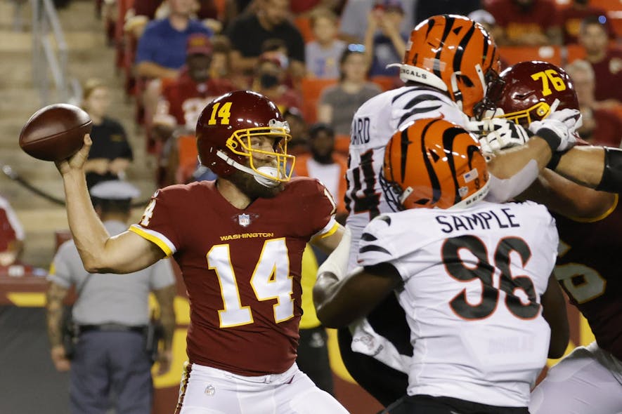
At 6'3" and 272 pounds, Cameron is a very large Sample

The performance of our "low ypc" backs above highlights one of the key facts of regression to the mean: outlier performances are significantly more likely over small samples. This informs the selection of our groups-- because of the small samples provided by an NFL season, the most extreme values in any given statistic are most likely chance-driven outliers. 

This also informs the nature of our predictions. If I flip a coin that's weighted to land on heads 60% of the time, that means there's still a 40% chance it lands on tails. Given those odds, landing on tails wouldn't be very surprising at all. But if I flipped the same coin a million times, the odds of seeing tails come up more often than heads dwindles down to nothing.

Already a subscriber?

Continue reading this content with a PRO subscription.

Similarly, if I single out one outlier player for regression, I'm more likely to be right than wrong... but I still might have a 40% chance of being wrong. If I bundle a bunch of outlier players together, though, the odds of being wrong fall substantially. Same idea behind running predictions for multiple weeks-- the longer the better, though I do like to have a clearly defined endpoint to make it easier to register our wins and losses for the year.

This idea that variance evens out over larger samples is one of the key insights of high-volume fantasy football players. Why do top DFS players compete with so many different lineups every week? The answer is not, as is commonly believed because it increases their expected return on investment. Indeed, every DFS player has a "best" lineup, a lineup that they think is most likely to win that week, and every other lineup that player submits actually decreases expected payout (because it's a worse lineup than the best lineup).

So why submit so many different lineups? Because outlier performances are significantly more likely over small samples. By using 20 lineups in a week, top players reduce the amount of money they'd be expected to win, but they also reduce the chances of a single injury or bad performance wiping out their entire bankroll, and that's a worthwhile trade.

In larger tournaments, they might estimate their best lineup has a 1% chance of winning while their second-best lineup only has a 0.9% shot. But if they only played the 1% lineup, it would take 69 weeks (about four years) before they passed the point where their odds of winning at least one tournament were greater than 50%. By using both the 1% and 0.9% lineup, that falls to 37 weeks. If they added a lineup with a 0.8% chance of winning, that falls to 26 weeks. The lineups might be worse, but the more you enter, the quicker luck tends to strike.

(Of course, larger samples reduce variance in both directions. A DFS player who submits 20 lineups is far less likely to lose their entire bankroll, but they're far less likely to double it, too. And multi-entering big tournaments reduces the time until they finally win one but greatly increases the cost, decreasing the proportionate return on investment.)

Why is it that three weeks at the beginning of the year don't give us enough information to outperform ADP, but five weeks do? Because three weeks is too small of a sample for the outlier performances to have all washed out sufficiently, and five weeks is not.

The fact that outliers are more common on smaller samples tends to manifest in our results over time, too. The biggest leads we ever see from Group B almost always occur in the first or second week of our prediction when the samples are still small (as we've seen on both of our predictions so far this year.) On the other hand, when Group B does trail, it also tends to occur in the week or two immediately after the prediction.

And while I always report the size of the lead in either direction (that darn accountability thing again), this is often misleading. A 20% lead over four weeks is significantly more impressive (as in "less likely to happen by chance alone") than a 30% lead over one week. (Consider: if Group B leads Group A by 30% after one week, then a 30% edge by Group A in the next week will erase that lead. If Group B leads Group A by 20% after four weeks, then a 30% edge by Group A in the next week will still leave Group B 10% ahead, provided all sample sizes are roughly equal.)

We've seen this in our first prediction this year, too. Last week, Group B led Group A by 27%. This week, they lead by 19%. Did Group A narrow the gap? Hardly; Group B outscored Group A last week, they just did so by less than the amount they'd been outscoring Group A so far, which reduced the "size" of the lead. But last week still left Group A more points behind with fewer games remaining to make those points up. The lead may be "shrinking", but Group A certainly isn't catching up.

Here's another illustration of the impact of small differences over large samples. For those of you who have been watching football for long enough, you probably remember the 2004 NFL season. The 2003 season closed with the New England Patriots beating the Indianapolis Colts 24-14 in a game that wasn't as close as the final score might suggest. The Colts complained that the Patriots' defensive backs were hitting receivers more than five yards beyond the line of scrimmage, which violated the rules as written, and the referees let it slide.

Over the offseason, the NFL's competition committee decided it would place a "point of emphasis" on ensuring officiating crews began calling contact downfield in line with the rules as written. NFL defenses adjusted by being less physical in coverage and passing offenses exploded, setting numerous records, headlined by Peyton Manning's own 49-touchdown season. After 2004, the NFL quietly dropped the point of emphasis, officiating crews went back to letting contact six or seven yards downfield slide, and offenses dropped off again.

In 2003, the league-wide average for yards per pass attempt was 6.6. In 2004, it spiked all the way to 7.1. In 2005, it fell back down to 6.8. (For context, yards per attempt in each of the last three seasons has been 7.0, 7.0, and 7.1; the 2004 season was essentially 15-20 years ahead of its time.)

That was it. Three-tenths, five-tenths of a yard per pass attempt, that was the difference between a stifling defensive environment and a wide-open offensive environment. When an offense dropped back to pass in 2004, the result was approximately 7.5% better than when it dropped back to pass in 2003.

On a player level, a 0.3-0.5 extra yards per attempt isn't a big difference. So far this season, Jared Goff leads Jayden Daniels by 0.4 yards per attempt, though I suspect most would say Daniels has had the better year.

But that's a difference of half a yard on a couple of hundred attempts. This was a difference of half a yard... over 16,354 attempts. Despite attempting 139 fewer passes, the league as a whole passed for an extra 5169 yards in 2004. It conjured an entire 1984 Dan Marino out of thin air. Over a sample that large, even a small change is massive.

What does this mean for us? It means if we want to make a sure profit in fantasy football by betting on regression to the mean, we're going to need to place a lot of bets. Trading away one player or acquiring another simply because they have a profile that suggests regression is a positive move in expectation, but the range of possible outcomes is massive. It could work out really well, it could work out terribly. Weighted coins still flip tails rather frequently.

It also means that the more bets we place on regression to the mean, the more our upside becomes capped. With larger samples, the odds of hitting big on every bet decline. The larger our sample, the smaller our potential rate of return.

But just like top DFS players, when you have a genuine edge, it can often make sense to turn to safer profits over gambling on the potential to strike it big while leaving yourself fully exposed to the consequences if the flip doesn't go your way.


Photos provided by Imagn Images

More by Adam Harstad


Dynasty, in Theory: Do the Playoffs Matter?

Adam Harstad

Should we include playoff performances when evaluating players?

01/18/25 Read More
 

Odds and Ends: Divisional Round

Adam Harstad

Examining past trends to predict the future.

01/17/25 Read More
 

Odds and Ends: Wild Card Weekend

Adam Harstad

Examining the playoff futures and correctly predicting the Super Bowl winner.

01/10/25 Read More
 

Dynasty, in Theory: Evaluating Rookie Receivers

Adam Harstad

Revisiting this year's rookies through the lens of the model

01/09/25 Read More
 

Dynasty, in Theory: Consistency is a Myth

Adam Harstad

Some believe consistency helps you win. (It doesn't.)

01/04/25 Read More
 

Odds and Ends: Week 18

Adam Harstad

How did we do for the year? Surprisingly well!

01/02/25 Read More